Take-home_Exercise2

Author

Zou Jiaxun

Published

May 2, 2024

1. Background

This project is a continuation from Take-take Exercise 1. The objective is to analyse the charts by applying the data visualisation design principles and best practices, and to improve on one of the submissions prepared by a fellow classmate. ZHANG CHENBIN in Take-home Exercise 1 submission will be selected to have some comments and try to improve it.

I’m going to Judge you!

2. Review & Enhance

Load the package and prepare the cleaned data first:

Click to view code
pacman::p_load(tidyverse, lubridate, patchwork, zoo, ggiraph, plotly, gifski, gapminder, patchwork, DT, colorspace, ggridges, ggthemes, ggdist, dplyr, cowplot)
data1 = read_csv("2023Q1.csv")
data2 = read_csv("2023Q2.csv")
data3 = read_csv("2023Q3.csv")
data4 = read_csv("2023Q4.csv")
data5 = read_csv("2024Q1.csv")
data <- bind_rows(data1, data2, data3, data4, data5)

glimpse(data)

data_cleaned <- data %>%
  mutate(
    `Sale Date` = dmy(`Sale Date`),  # Ensuring we're using the exact column name from the dataset
    `Area (SQM)` = as.numeric(gsub(",", "", `Area (SQM)`)),  # Keeping the variable names as they are in the dataset
    `Unit Price ($ PSM)` = as.numeric(gsub("\\$", "", gsub(",", "", `Unit Price ($ PSM)`)))  # Properly referencing the variable
  )

data_cleaned <- data_cleaned %>%
  mutate(
    `Area (SQM)` = ifelse(is.na(`Area (SQM)`), 0, `Area (SQM)`)  # Dealing with NA values
  )

data_cleaned <- data_cleaned %>%
  mutate(
    Area_Category = cut(
      `Area (SQM)`,
      breaks = c(0, 100, 200, 300, 400, Inf),  
      labels = c("<100", "100-200", "200-300", "300-400", ">400"),
      include.lowest = TRUE  
    )
  )

Chenbin choosed and divided the data before the graph occured is weired, what variables he choosed are “Sale Data”, “Area (SQM)”, “Unit Price ($PSM)”.

2.1 First Analysis - Quarterly Housing Prices by Area Category

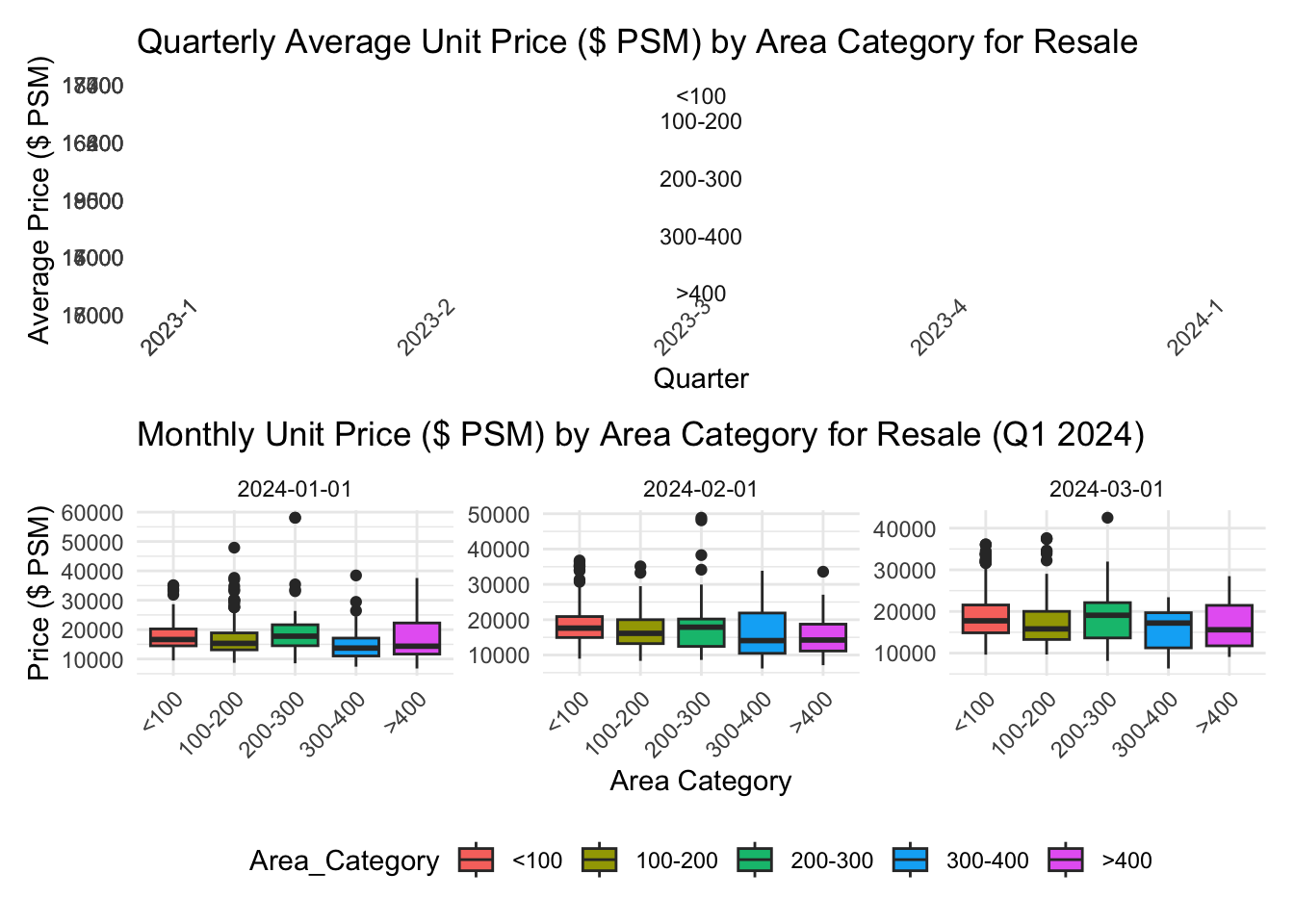
The original plot handled average price before utilizing 4 plots to show different Area range’s average Unit Price, and used three plots to present Q1 2024 situation.

Rows: 26,806
Columns: 21
$ `Project Name`                <chr> "THE REEF AT KING'S DOCK", "URBAN TREASU…
$ `Transacted Price ($)`        <dbl> 2317000, 1823500, 1421112, 1258112, 1280…
$ `Area (SQFT)`                 <dbl> 882.65, 882.65, 1076.40, 1033.34, 871.88…
$ `Unit Price ($ PSF)`          <dbl> 2625, 2066, 1320, 1218, 1468, 1767, 1095…
$ `Sale Date`                   <chr> "01 Jan 2023", "02 Jan 2023", "02 Jan 20…
$ Address                       <chr> "12 HARBOURFRONT AVENUE #05-32", "205 JA…
$ `Type of Sale`                <chr> "New Sale", "New Sale", "New Sale", "New…
$ `Type of Area`                <chr> "Strata", "Strata", "Strata", "Strata", …
$ `Area (SQM)`                  <dbl> 82.0, 82.0, 100.0, 96.0, 81.0, 308.7, 42…
$ `Unit Price ($ PSM)`          <dbl> 28256, 22238, 14211, 13105, 15802, 19015…
$ `Nett Price($)`               <chr> "-", "-", "-", "-", "-", "-", "-", "-", …
$ `Property Type`               <chr> "Condominium", "Condominium", "Executive…
$ `Number of Units`             <dbl> 1, 1, 1, 1, 1, 1, 1, 1, 1, 1, 1, 1, 1, 1…
$ Tenure                        <chr> "99 yrs from 12/01/2021", "Freehold", "9…
$ `Completion Date`             <chr> "Uncompleted", "Uncompleted", "Uncomplet…
$ `Purchaser Address Indicator` <chr> "HDB", "Private", "HDB", "HDB", "HDB", "…
$ `Postal Code`                 <chr> "097996", "419535", "269343", "269294", …
$ `Postal District`             <chr> "04", "14", "27", "27", "28", "19", "10"…
$ `Postal Sector`               <chr> "09", "41", "26", "26", "79", "54", "27"…
$ `Planning Region`             <chr> "Central Region", "East Region", "North …
$ `Planning Area`               <chr> "Bukit Merah", "Bedok", "Yishun", "Yishu…

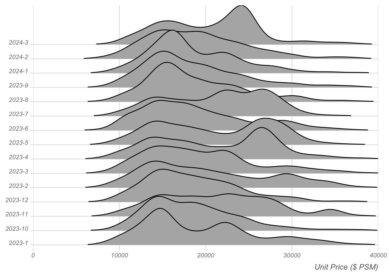
Instead of relying on average unit price, utilizing the frequency of distributed area (in square meters) can better illustrate purchasing power and market potential, particularly when the total number of transactions is unknown. Additionally, for a clearer understanding of specific Q1 2024 sales data, opting for a density plot can effectively visualize the distribution of unit prices.

2.2.Comparative Analysis of Transaction Volumes and Pricing Across Real Estate Projects

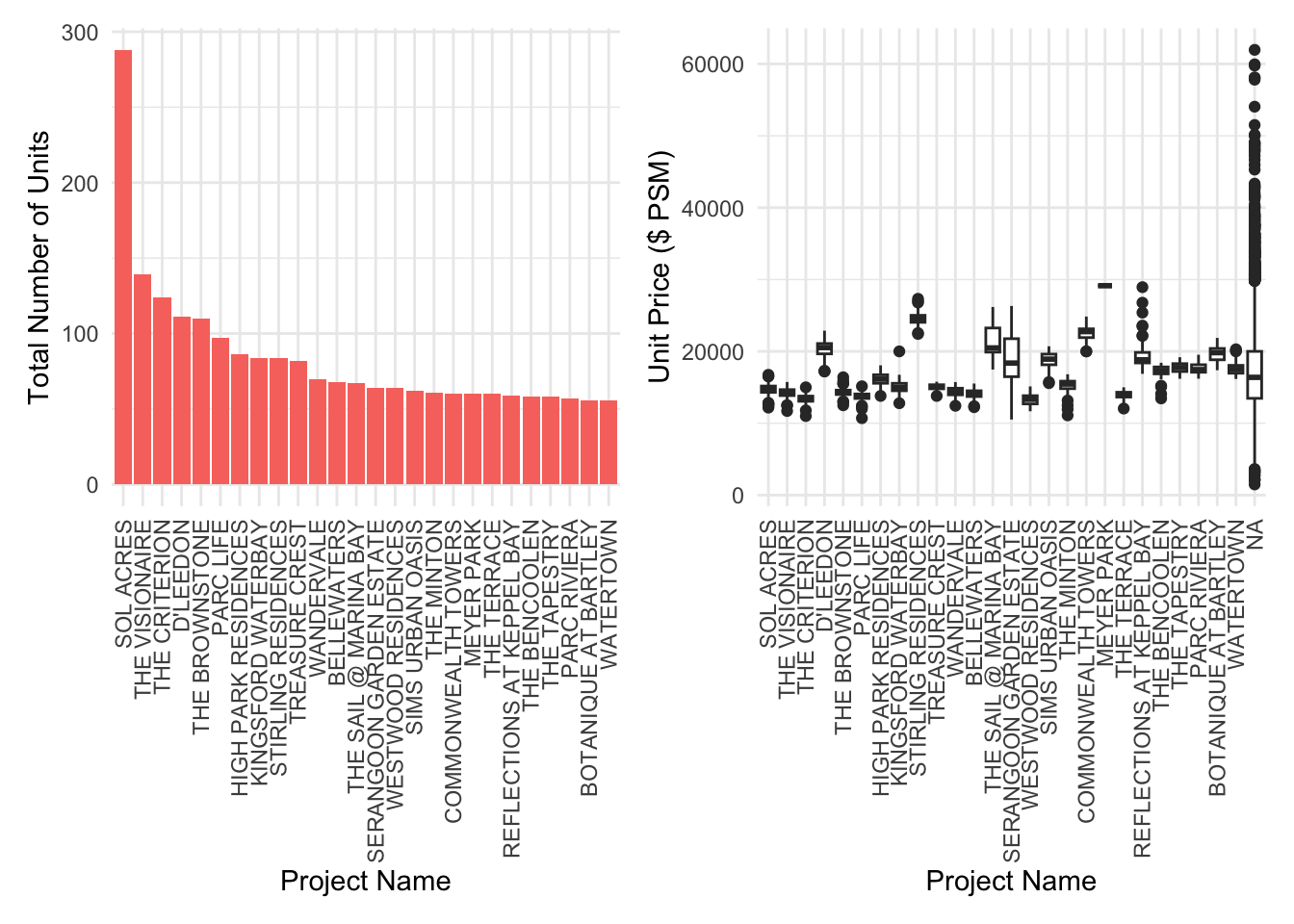
Chenbin employed two plots: one depicting the frequency of various projects and the other illustrating the purchase situation across different projects.

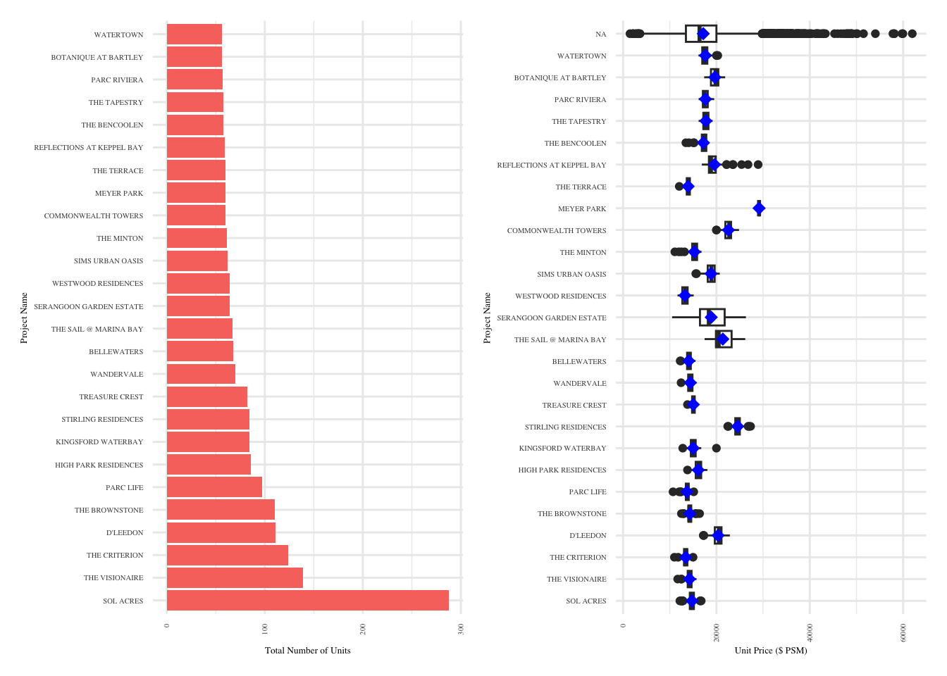
To broaden the scope and facilitate comparison between project categories, we can utilize a flip in plot orientation. Additionally, incorporating mean statistics can effectively convey Chenbin’s intended presentation in the aforementioned plots.

3.Conclusion

The data from the first quarter of 2024 shows that “Sol Acres” significantly leads in resale volumes, hinting at its market desirability, possibly due to a balance of affordability and attractive amenities. This project’s success may be a key indicator for those seeking value-for-money investments. In contrast, luxury segments like “The Sail @ Marina Bay” exhibit a wide price range, indicating a market for buyers with a taste for exclusivity and willingness to pay a premium for distinctive features.

For Consumers: Buyers should align their choices with their priorities: affordability may lead them to high-volume projects, while unique, high-quality features could draw them towards premium segments. When considering investment, a diversified approach that includes stable, high-volume properties and selective, high-value opportunities may offer balanced returns.

4.Reference